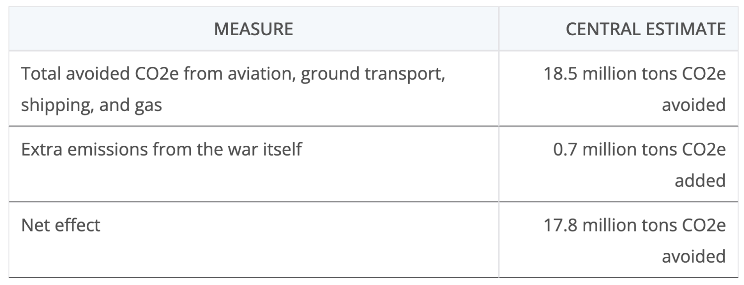
The idea that Donald Trump might be an accidental climate warrior rests on a narrow and uncomfortable observation. Wars, price shocks, and trade disruptions can suppress fossil fuel demand in the short term. That suppression shows up as lower emissions in the ledger. It does not come from better systems. It comes from stress applied to a system that depends on continuous flows of oil, gas, and coal. The Strait of Hormuz crisis provides a recent example that is large enough to analyze across multiple sectors with some rigor. Table of estimates of avoided CO2e by author. This is a scenario analysis, not a measured inventory. The numbers are counterfactual, comparing what likely would have happened without the disruption to what appears to have happened during it. Each sector is modeled separately using standard proxies. The results are presented as ranges with central estimates. Some sectors exhibit true demand destruction, while others shift activity in time. The goal is order of magnitude correctness rather than false precision. The key is to understand direction, scale, and where the uncertainties sit. The Strait of Hormuz is a systems node. It is a conduit for oil and LNG, a corridor for aviation routes, and a determinant of shipping flows and fuel prices. A disruption there propagates through aviation, road transport, shipping, and natural gas markets with different response functions. Treating those sectors with a single elasticity would be incorrect. Each has to be examined on its own terms. Aviation is the cleanest case because activity disappears rather than shifts. Cirium reported that before the conflict March 2026 had been expected to deliver about 5.6% global capacity growth, but in the first 22 days of the conflict global flown ASKs were down 2.5% year over year, while Middle East carrier capacity fell 56.5%. That is a very large gap between expected and actual activity, concentrated in a part of the network that carries a disproportionate share of long haul traffic. Using a global baseline of roughly 6.1 billion aircraft kilometers per month, derived from about 106,000 flights per day and an average stage length near 1,850 km, the disruption likely removed about 215 million to 365 million aircraft kilometers relative to expectation. That is about 3.5% to 6% of expected flying. Fuel intensity for the lost flying is higher than the global average because long haul Middle Eastern hub operations dominate. Using 5.5 to 7.5 kg of jet fuel per aircraft kilometer and applying a 10% to 25% penalty for longer rerouted flights that still operated, the avoided jet fuel burn comes out to about 0.9 million to 2.5 million tons, with a central estimate near 1.5 million tons. Using the standard factor of 3.16 tons of CO2 per ton of jet fuel, that corresponds to about 2.8 million to 7.9 million tons of direct CO2 avoided, centered near 4.7 million tons. Aviation also has non CO2 warming effects from contrails and NOx. Those matter, but they are uncertain and depend on route, altitude, weather, and metric. A broad multiplier approach yields a rough CO2e range of about 4.8 million to 23.7 million tons, with a midpoint around 11 million tons, but that should be treated as indicative rather than as a strict inventory. The direct CO2 estimate is the more defensible core result. Road transport responds differently. Global road fuel demand is about 45% of total oil demand. With global oil demand around 105 million barrels per day, road fuels are roughly 47 million barrels per day. Price shocks feed through to retail fuel prices with delays and regional variation. Reuters also reported work from home policies, driving curbs, and other conservation measures during the shock. That means the road estimate should be read as suppressed road fuel demand associated with the crisis, not as a clean behavioral response to pump prices alone. A reasonable effective global retail price increase over the month is about 5% to 15%, with a central estimate near 9%. Short run elasticity for road fuel demand is low. Modern estimates suggest a range of about -0.03 to -0.09 for a one month period. Using those values yields suppressed demand of about 0.07 to 0.64 million barrels per day, with a central estimate near 0.25 million barrels per day. Over 30 days, that is about 2 million to 19 million barrels avoided, with a midpoint near 8 million barrels. Converting using standard fuel densities gives about 0.26 million to 2.38 million tons of gasoline and diesel avoided, with a central estimate near 0.95 million tons. Using direct combustion factors expressed on a mass basis, about 3.11 tons of CO2 per ton of gasoline and about 3.19 tons of CO2 per ton of diesel, the avoided direct emissions are about 0.84 million to 7.6 million tons of CO2, centered near 3.0 million tons. On a lifecycle basis, including upstream emissions, the range is about 1.15 million to 10.36 million tons CO2e, centered near 4.1 million tons. That broader figure is useful for context, but the direct CO2 estimate remains the cleaner comparison with other sectors. Shipping is the contrast case. Ships at anchor burn far less fuel than ships underway, but much of the activity is delayed rather than destroyed. The right model is ship days, not ton miles. Reuters reported only seven ships transiting Hormuz in one 24 hour period versus about 140 normally, and hundreds of tankers and other ships were delayed. Underway fuel burn for large tankers ranges from about 30 to 65 tons per day. Hoteling loads at anchor range from about 4 to 14 tons per day. The difference, roughly 20 to 50 tons per day, is the gross saving when a ship is delayed. Using a range of 120 to 220 tanker equivalents delayed over a 31 day period gives about 0.08 million to 0.35 million tons of bunker fuel not burned during the disruption window, with a central estimate near 0.17 million tons. Including other vessel types adds some additional gross savings. The net effect is much smaller. Cargo still moves later, and rerouting increases fuel burn elsewhere. Applying a clawback of 50% to 90% for deferred voyages and rerouting reduces the net avoided bunker fuel to about 0.01 million to 0.21 million tons, with a central estimate around 0.05 to 0.075 million tons. Using about 3.12 tons CO2 per ton of fuel, that corresponds to about 0.03 million to 0.66 million tons of direct CO2, centered near 0.2 million tons. On a lifecycle basis, about 3.8 tons CO2e per ton of fuel gives roughly 0.03 million to 0.85 million tons CO2e, centered near 0.25 million tons. Shipping shows clearly that not all disruptions eliminate emissions. Many shift them in time and space. It is also one of the least certain sectors because the gross effect is easy to understand while the net effect depends on later behavior. Natural gas is more complex still. Global demand is about 4,374 bcm per year, or about 364 bcm per month. Spot prices rose sharply, with Asian LNG prices up over 100% and European prices up over 70% in some periods, but retail pass through was muted in many markets and contract structures shielded some buyers. A reasonable effective global price shock is about 5% to 18%, with a central estimate near 9%. Short run global elasticity is modest, about -0.02 to -0.06. Applying those values gives suppressed demand of about 0.36 bcm to 3.94 bcm, with a central estimate near 1.3 bcm. Each bcm of gas corresponds to about 1.95 million tons of CO2 when combusted. That yields about 0.7 million to 7.7 million tons of direct CO2 avoided, centered near 2.6 million tons. Including upstream emissions gives about 0.85 million to 9.2 million tons CO2e, centered near 3.1 million tons. The key caveat is substitution. Gas displaced by price shocks can be replaced by coal or oil, reducing or reversing net emissions benefits. This sector has the largest uncertainty in terms of net climate impact. Lower gas use is real. Lower economy wide emissions are not guaranteed. Against these avoided emissions, there are additional emissions caused by the conflict itself. Military operations burn fuel. Public data indicates at least 13,000 combat flights in one U.S. operation alone. Using a blended estimate of 8 to 20 tons CO2e per flight yields about 0.1 million to 0.26 million tons CO2e. Naval escorts add another roughly 0.04 million to 0.11 million tons. Extending to all belligerents gives a plausible range of about 0.2 million to 0.9 million tons CO2e. Damage to fossil infrastructure adds more. Fires and flaring at gas and oil facilities likely contributed about 0.1 million to 0.4 million tons CO2e, with higher uncertainty if methane releases occurred. A reasonable combined estimate for war caused emissions is about 0.3 million to 1.3 million tons CO2e, with a midpoint near 0.7 million tons. If the analysis is kept to the narrowest and most comparable ledger, direct emissions, the picture is relatively clear. Summing the avoided direct CO2 across aviation, road transport, shipping, and natural gas gives about 4.4 million to 23.8 million tons, with a central estimate near 10.5 million tons. Subtracting the estimated war caused emissions yields a net range of about 3.1 million to 23.5 million tons of avoided emissions, centered near 9.8 million tons. That is the strongest numerical conclusion in the piece because it compares more similar things. A broader CO2e framing can be added, but it should be treated with caution. Aviation CO2e in this discussion includes non CO2 warming effects. Road, shipping, and gas CO2e are mostly lifecycle supply chain additions. War caused emissions are mostly direct operational fuel burn plus fires and some possible methane releases. Those are not identical accounting boundaries. Even so, as an indicative side calculation, the broader avoided range comes out to about 6.8 million to 44.1 million tons CO2e, with a central estimate near 18.5 million tons CO2e. After subtracting the war caused emissions, the indicative net range is about 5.5 million to 43.8 million tons CO2e, centered near 17.8 million tons. That is useful for illustrating scale, but it should not be mistaken for a single harmonized inventory. The uncertainty in these estimates is not trivial. Measurement uncertainty comes from limited real time data and reliance on proxies. Behavioral uncertainty comes from elasticity assumptions and policy responses. System uncertainty comes from fuel switching, rerouting, and deferred activity. Aviation is the most reliable estimate. Road transport is moderately reliable. Shipping net and natural gas net have lower confidence due to time shifting and substitution. The value of the exercise is not a false claim to precision. It is that the ranges, despite their spread, point in the same direction. The distribution of impacts across countries is not uniform. Spain weathered the shock better than many because it has built a system with a high share of wind, solar, and hydro supported by a capable grid. Its exposure to imported gas at the margin is lower. Pakistan performed better than expected because of a rapid expansion of distributed solar that reduced its need for LNG at peak times. In both cases, the mechanism is the same. Lower dependence on imported fossil fuels reduces vulnerability to price and supply shocks. This pattern extends globally. China has built more than 2,200 GW of wind, water, and solar capacity. Europe has over 1,000 GW. India is adding tens of gigawatts per year and now exceeds 250 GW. The United States, with about 380 GW, lags relative to its economic size and capability. When normalized by GDP, China and India are building clean capacity at several times the rate of the United States. These are not abstract climate metrics. They are indicators of future resilience to shocks like Hormuz. The phrase accidental climate warrior captures a narrow truth. Policies and actions that increase conflict, disrupt trade, and drive up fossil fuel prices can reduce emissions for a time. They do so by suppressing demand. The estimates here suggest that effect can be material, on the order of 10 million tons of CO2 or more over a month on a direct emissions basis. But this is not a pathway to a stable climate. It is a consequence of disruption. When prices normalize and activity resumes, emissions return unless underlying systems have changed. The deeper lesson is about systems. Fossil dependent systems break under stress. Electrified systems bend. Spain and Pakistan illustrate two paths to reduced exposure. China and India show the scale at which that transition is occurring. The United States shows that capability alone does not guarantee progress. If emissions fall because of conflict and price shocks, it is a sign of fragility, not success. The path that matters is the one that reduces dependence on fuels that must be imported, shipped, and burned, replacing them with electricity that can be generated domestically from wind, water, and solar.